Predator prey model application examples. Equilibrium predator-prey. Simulation modeling of the "Predator-Prey" system
COMPUTER MODEL "PREDATOR-Prey"
Kazachkov Igor Alekseevich 1 , Guseva Elena Nikolaevna 2
1 Magnitogorsk State Technical University them. G.I. Nosova, Institute of Construction, Architecture and Art, 5th year student
b Magnitogorsk State Technical University G.I. Nosova, Institute of Energy and Automated Systems, Candidate of Pedagogical Sciences, Associate Professor of the Department of Business Informatics and Information Technologies
annotation
This article is devoted to the review of the computer model "predator-prey". The study allows us to state that ecological modeling plays a huge role in the study of the environment. This issue is multifaceted.
COMPUTER MODEL "PREDATOR-VICTIM"
Kazatchkov Igor Alekseevich 1 , Guseva Elena Nikolaevna 2
1 Nosov Magnitogorsk State Technical University, Civil Engineering, Architecture and Arts Institute, student of the 5th course
2 Nosov Magnitogorsk State Technical University, Power Engineering and Automated Systems Institute, PhD in Pedagogical Science, Associate Professor of the Business Computer Science and Information Technologies Department
Abstract
This article provides an overview of the computer model "predator-victim". The study suggests that environmental simulation plays a huge role in the study of the environment. This problem is multifaceted.
Ecological modeling is used to study the environment around us. Mathematical models are used in cases where there is no natural environment and no natural objects, it helps to predict the impact various factors to the object under study. This method takes over the functions of checking, constructing and interpreting the results. On the basis of such forms, ecological modeling deals with the assessment of changes in the environment around us.
At the moment, such forms are used to study the environment around us, and when it is required to study any of its areas, then mathematical modeling is used. This model makes it possible to predict the influence of certain factors on the object of study. At one time, the “predator-prey” type was proposed by such scientists as: T. Malthus (Malthus 1798, Malthus 1905), Verhulst (Verhulst 1838), Pearl (Pearl 1927, 1930), as well as A. Lotka (Lotka 1925, 1927 ) and V. Volterra (Volterra 1926). These models reproduce the periodic oscillatory regime that occurs as a result of interspecies interactions in nature.
One of the main methods of cognition is modeling. In addition to being able to predict changes in the environment, it also helps to find the best way to solve a problem. For a long time, mathematical models have been used in ecology in order to establish patterns, trends in the development of populations, and help to highlight the essence of observations. The layout can serve as a sample behavior, object.
When recreating objects in mathematical biology, predictions of various systems are used, special individualities of biosystems are provided for: the internal structure of an individual, life support conditions, the constancy of ecological systems, thanks to which the vital activity of systems is saved.
The advent of computer simulation has greatly pushed the frontier of research capability. There was a possibility of multilateral implementation of difficult forms that do not allow analytical study, new trends appeared, as well as simulation modeling.
Let's consider what is the object of modeling. “The object is a closed habitat where the interaction of two biological populations takes place: predators and prey. The process of growth, extinction and reproduction takes place directly on the surface of the environment. Prey feed on the resources that are present in the environment, while predators feed on prey. At the same time, nutritional resources can be both renewable and non-renewable.
In 1931, Vito Volterra derived the following laws of the predator-prey relationship.
The law of the periodic cycle - the process of destruction of the prey by a predator often leads to periodic fluctuations in the number of populations of both species, depending only on the growth rate of carnivores and herbivores, and on the initial ratio of their numbers.
Law of conservation of averages - the average abundance of each species is constant, regardless of the initial level, provided that the specific rates of population increase, as well as the efficiency of predation, are constant.
The law of violation of averages - with a reduction in both species in proportion to their number, the average population of prey increases, and predators - decreases.
The predator-prey model is a special relationship between the predator and the prey, as a result of which both benefit. The most healthy and adapted individuals to the environmental conditions survive, i.e. All this is due to natural selection. In an environment where there is no opportunity for reproduction, the predator will sooner or later destroy the prey population, after which it will die out itself.
There are many living organisms on earth, which, under favorable conditions, increase the number of relatives to enormous proportions. This ability is called: the biotic potential of the species, i.e. an increase in the population of a species over a given period of time. Each species has its own biotic potential, for example large species organisms per year can increase by only 1.1 times, in turn, organisms of smaller species, such as crustaceans, etc. can increase their appearance up to 1030 times, but bacteria are even larger. In any of these cases, the population will grow exponentially.
Exponential population growth is a geometric progression of population growth. This ability can be observed in the laboratory in bacteria, yeast. In non-laboratory conditions, exponential growth can be seen in locusts or other insect species. Such an increase in the number of the species can be observed in those places where it has practically no enemies, and there is more than enough food. Eventually the growth of the species, after the population increased for a short time, the population growth began to decline.
Consider a computer model of mammalian reproduction on the example of the Lotka-Volterra model. Let two species of animals live in a certain area: deer and wolves. Mathematical model of population change in the model Trays-Volterra:
The initial number of victims is xn, the number of predators is yn.
Model parameters:
P1 is the probability of meeting with a predator,
P2 is the growth rate of predators at the expense of prey,
d is the predator mortality rate,
a is the increase in the number of victims.
IN learning task the following values were set: the number of deer was 500, the number of wolves was 10, the growth rate of deer was 0.02, the growth rate of wolves was 0.1, the probability of meeting a predator was 0.0026, the growth rate of predators due to prey was 0.000056. Data are calculated for 203 years.
Exploring influence the growth rate of victims for the development of two populations, the remaining parameters will be left unchanged. In Scheme 1, an increase in the number of prey is observed, and then, with some delay, an increase in predators is observed. Then the predators knock out the prey, the number of prey drops sharply, followed by the decrease in the number of predators (Fig. 1).

Figure 1. Population size with low birth rates among victims
Let us analyze the change in the model by increasing the birth rate of the victim a=0.06. In Scheme 2, we see a cyclic oscillatory process leading to an increase in the number of both populations over time (Fig. 2).

Figure 2. Population size at the average birth rate of the victims
Let's consider how the dynamics of populations will change with a high value of the birth rate of the victim a = 1.13. On fig. 3, there is a sharp increase in the number of both populations, followed by extinction of both prey and predator. This is due to the fact that the population of victims has increased to such an extent that resources have begun to run out, as a result of which the victim is dying out. The extinction of predators is due to the fact that the number of victims has decreased and the predators have run out of resources for existence.
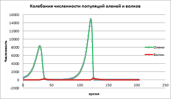
Figure 3. Populations with high birth rates in prey
Based on the analysis of the computer experiment data, it can be concluded that computer modelling allows us to predict the number of populations, to study the influence of various factors on population dynamics. In the above example, we investigated the predator-prey model, the effect of the birth rate of prey on the number of deer and wolves. A small increase in the population of prey leads to a small increase in prey, which after a certain period is destroyed by predators. A moderate increase in the prey population leads to an increase in the size of both populations. A high increase in the population of prey first leads to a rapid increase in the population of prey, this affects the increase in the growth of predators, but then the breeding predators quickly destroy the deer population. As a result, both species become extinct.
Federal Agency for Education
State educational institution
higher professional education
"Izhevsk State Technical University"
Faculty of Applied Mathematics
Department "Mathematical modeling of processes and technologies"
Course work
in the discipline "Differential Equations"
Topic: "Qualitative study of the predator-prey model"
Izhevsk 2010
INTRODUCTION
1. PARAMETERS AND MAIN EQUATION OF THE PREDATOR- PREY MODEL
2.2 Generalized models of Voltaire of the "predator-prey" type.
3. PRACTICAL APPLICATIONS OF THE PREDATOR- PREY MODEL
CONCLUSION
BIBLIOGRAPHY
INTRODUCTION
Currently, environmental issues are of paramount importance. An important step in solving these problems is the development of mathematical models of ecological systems.
One of the main tasks of the ecology of pa present stage is the study of the structure and functioning of natural systems, the search for general patterns. Mathematics, which contributed to the formation of mathematical ecology, had a great influence on ecology, especially its sections such as theory differential equations, stability theory and optimal control theory.
One of the first works in the field of mathematical ecology was the work of A.D. Trays (1880 - 1949), who first described the interaction of different populations, related relationships predator is prey. A great contribution to the study of the predator-prey model was made by V. Volterra (1860 - 1940), V.A. Kostitsyn (1883-1963) At present, the equations describing the interaction of populations are called the Lotka-Volterra equations.
The Lotka-Volterra equations describe the dynamics of average values - population size. At present, on their basis, more general models of interaction between populations, described by integro-differential equations, are constructed, controlled predator-prey models are being studied.
One of the important problems of mathematical ecology is the problem of the stability of ecosystems and the management of these systems. Management can be carried out with the aim of transferring the system from one stable state to another, with the aim of using it or restoring it.
1. PARAMETERS AND MAIN EQUATION OF THE PREDATOR- PREY MODEL
Attempts to mathematically model the dynamics of both individual biological populations and communities that include interacting populations various kinds have been undertaken for a long time. One of the first growth models for an isolated population (2.1) was proposed back in 1798 by Thomas Malthus:
This model is set by the following parameters:
N - population size;
The difference between birth and death rates.
Integrating this equation we get:
![]() , (1.2)
, (1.2)
where N(0) is the population size at the moment t = 0. Obviously, the Malthus model for > 0 gives an infinite population growth, which is never observed in natural populations, where the resources that ensure this growth are always limited. Changes in the number of populations of flora and fauna cannot be described by a simple Malthusian law; many interrelated reasons influence the dynamics of growth - in particular, the reproduction of each species is self-regulated and modified so that this species is preserved in the process of evolution.
The mathematical description of these regularities is carried out by mathematical ecology - the science of the relationship of plant and animal organisms and the communities they form with each other and with environment.
The most serious study of models of biological communities, which include several populations of different species, was carried out by the Italian mathematician Vito Volterra:
 ,
,
where is the population size;
Coefficients of natural increase (or mortality) of the population; - coefficients of interspecies interaction. Depending on the choice of coefficients, the model describes either the struggle of species for a common resource, or interaction of the predator-prey type, when one species is food for another. If in the works of other authors the main attention was paid to the construction of various models, then V. Volterra conducted a deep study of the constructed models of biological communities. It is from the book of V. Volterra, in the opinion of many scientists, that modern mathematical ecology began.
2. QUALITATIVE STUDY OF THE ELEMENTARY MODEL "PREDATOR- PREY"
2.1 Predator-prey trophic interaction model
Let us consider the model of trophic interaction according to the "predator-prey" type, built by W. Volterra. Let there be a system consisting of two species, of which one eats the other.
Consider the case when one of the species is a predator and the other is a prey, and we will assume that the predator feeds only on the prey. We accept the following simple hypothesis:
Prey growth rate;
Predator growth rate;
Prey population;
Predator population size;
Coefficient of natural increase of the victim;
The rate of prey consumption by the predator;
Predator mortality rate in the absence of prey;
Coefficient of “processing” of the prey biomass by the predator into its own biomass.
Then the population dynamics in the predator-prey system will be described by the system of differential equations (2.1):
 (2.1)
(2.1)
where all coefficients are positive and constant.
The model has an equilibrium solution (2.2):
According to model (2.1), the proportion of predators in the total mass of animals is expressed by formula (2.3):
 (2.3)
(2.3)
An analysis of the stability of the equilibrium state with respect to small perturbations showed that the singular point (2.2) is “neutrally” stable (of the “center” type), i.e., any deviations from equilibrium do not decay, but transfer the system into an oscillatory regime with an amplitude depending on the magnitude of the disturbance. The trajectories of the system on the phase plane have the form of closed curves located at different distances from the equilibrium point (Fig. 1).

Rice. 1 - Phase "portrait" of the classical Volterra system "predator-prey"
Dividing the first equation of system (2.1) by the second, we obtain differential equation (2.4) for the curve on the phase plane .
 (2.4)
(2.4)
Integrating this equation, we get:
![]() (2.5)
(2.5)
where is the constant of integration, where 
It is easy to show that the movement of a point along the phase plane will occur only in one direction. To do this, it is convenient to make a change of functions and , moving the origin of coordinates on the plane to a stationary point (2.2) and then introducing polar coordinates:
 (2.6)
(2.6)
In this case, substituting the values of system (2.6) into system (2.1), we have:
 (2.7)
(2.7)
Multiplying the first equation by and the second by and adding them, we get:
After similar algebraic transformations, we obtain the equation for:
The value , as can be seen from (4.9), is always greater than zero. Thus does not change sign, and the rotation is all time is running one way.
Integrating (2.9) we find the period:
When it is small, then equations (2.8) and (2.9) pass into the equations of an ellipse. The period of circulation in this case is equal to:
 (2.11)
Based on the periodicity of solutions of equations (2.1), we can obtain some corollaries. For this, we represent (2.1) in the form:
 (2.12)
and integrate over the period:
 (2.13)
Since the substitutions from and due to periodicity vanish, the averages over the period turn out to be equal to the stationary states (2.14):
 (2.14)
The simplest equations of the "predator-prey" model (2.1) have a number of significant drawbacks. Thus, they assume unlimited food resources for the prey and unlimited growth of the predator, which contradicts the experimental data. In addition, as can be seen from Fig. 1, none of the phase curves is highlighted in terms of stability. In the presence of even small perturbing influences, the trajectory of the system will go farther and farther from the equilibrium position, the amplitude of oscillations will increase, and the system will quickly collapse.
Despite the shortcomings of model (2.1), ideas about the fundamentally oscillatory nature of the dynamics of the "predator-prey" system have become widespread in ecology. Predator-prey interactions were used to explain such phenomena as fluctuations in the number of predatory and peaceful animals in hunting zones, fluctuations in populations of fish, insects, etc. In fact, fluctuations in numbers can be due to other reasons.
Let us assume that in the predator-prey system artificial destruction of individuals of both species takes place, and we will consider the question of how the destruction of individuals affects the average values of their numbers, if it is carried out in proportion to this number with proportionality coefficients and, respectively, for prey and predator. Taking into account the assumptions made, we rewrite the system of equations (2.1) in the form:
 (2.15)
We assume that , i.e., the coefficient of extermination of the victim is less than the coefficient of its natural increase. In this case, periodic fluctuations in numbers will also be observed. Let us calculate the average values of the numbers:
 (2.16)
Thus, if , then the average number of prey populations increases, and that of predators decreases.
Let us consider the case when the coefficient of prey extermination is greater than the coefficient of its natural increase, i.e. In this case ![]() for any , and, therefore, the solution of the first equation (2.15) is bounded from above by an exponentially decreasing function
for any , and, therefore, the solution of the first equation (2.15) is bounded from above by an exponentially decreasing function ![]() , i.e. at .
, i.e. at .
Starting from some moment of time t, at which , the solution of the second equation (2.15) also begins to decrease and tends to zero as . Thus, in the case of both species disappear.
2.1 Generalized Voltaire models of the "predator-prey" type
The first models of V. Volterra, of course, could not reflect all aspects of the interaction in the predator-prey system, since they were largely simplified in relation to real conditions. For example, if the number of predators is equal to zero, then it follows from equations (1.4) that the number of prey increases indefinitely, which is not true. However, the value of these models lies precisely in the fact that they were the basis on which mathematical ecology began to develop rapidly.
A large number of studies of various modifications of the predator-prey system have appeared, where more general models have been constructed that take into account, to one degree or another, the real situation in nature.
In 1936 A.N. Kolmogorov suggested using the following system of equations to describe the dynamics of the predator-prey system:
 , (2.17)
where decreases with an increase in the number of predators, and increases with an increase in the number of prey.
This system of differential equations, due to its sufficient generality, makes it possible to take into account the real behavior of populations and, at the same time, to carry out a qualitative analysis of its solutions.
Later in his work, Kolmogorov explored in detail a less general model:
 (2.18)
Various particular cases of the system of differential equations (2.18) have been studied by many authors. The table lists various special cases of the functions , , .
Table 1 - Different models of the "predator-prey" community
| Authors | |||
| Volterra Lotka | |||
| Gause | |||
| Pislow | |||
| Holing | |||
| Ivlev | |||
| Royama | |||
| Shimazu | |||
| May |
mathematical modeling predator prey
3. PRACTICAL APPLICATIONS OF THE PREDATOR- PREY MODEL
Let us consider a mathematical model of coexistence of two biological species (populations) of the "predator-prey" type, called the Volterra-Lotka model.
Let two biological species live together in an isolated environment. The environment is stationary and provides an unlimited amount of everything necessary for life to one of the species, which we will call the victim. Another species - a predator is also in stationary conditions, but feeds only on individuals of the first species. These can be crucians and pikes, hares and wolves, mice and foxes, microbes and antibodies, etc. For definiteness, we will call them crucians and pikes.
The following initial indicators are set:
Over time, the number of crucians and pikes changes, but since there are a lot of fish in the pond, we will not distinguish between 1020 crucians or 1021 and therefore we will also consider continuous functions of time t. We will call a pair of numbers (,) the state of the model.
Obviously, the nature of the state change (,) is determined by the values of the parameters. By changing the parameters and solving the system of equations of the model, it is possible to study the patterns of changes in the state of the ecological system over time.
In the ecosystem, the rate of change in the number of each species will also be considered proportional to its number, but only with a coefficient that depends on the number of individuals of another species. So, for crucian carp, this coefficient decreases with an increase in the number of pikes, and for pikes it increases with an increase in the number of carp. We will consider this dependence also linear. Then we get a system of two differential equations:

This system of equations is called the Volterra-Lotka model. Numerical coefficients , , - are called model parameters. Obviously, the nature of the state change (,) is determined by the values of the parameters. By changing these parameters and solving the system of equations of the model, it is possible to study the patterns of changes in the state of the ecological system.
Let's integrate the system of both equations with respect to t, which will vary from - the initial moment of time to , where T is the period for which changes occur in the ecosystem. Let in our case the period is equal to 1 year. Then the system takes the following form:
 ;
;
 ;
;
Taking = and = we bring similar terms, we obtain a system consisting of two equations:

Substituting the initial data into the resulting system, we get the population of pikes and crucian carp in the lake a year later:
PA88 system, which simultaneously predicts the probability of more than 100 pharmacological effects and mechanisms of action of a substance based on its structural formula. The efficiency of applying this approach to screening planning is about 800%, and the accuracy of computer prediction is 300% higher than that of experts.
So, one of the constructive tools for obtaining new knowledge and solutions in medicine is the method of mathematical modeling. The process of mathematization of medicine is a frequent manifestation of interpenetration scientific knowledge, increasing the effectiveness of treatment and preventive work.
4. Mathematical model "predators-prey"
For the first time in biology, a mathematical model of a periodic change in the number of antagonistic animal species was proposed by the Italian mathematician V. Volterra and his co-workers. The model proposed by Volterra was the development of the idea outlined in 1924 by A. Lotka in the book "Elements of Physical Biology". Therefore, this classical mathematical model is known as the "Lotka-Volterra" model.
Although antagonistic species relations are more complex in nature than in a model, they are nevertheless a good educational model on which to learn the basic ideas of mathematical modeling.
So, task: in some ecologically closed area two species of animals live (for example, lynxes and hares). Hares (prey) feed on plant foods, which are always available in sufficient quantities (this model does not take into account the limited resources of plant foods). Lynxes (predators) can only eat hares. It is necessary to determine how the number of prey and predators will change over time in such an ecological system. If the prey population increases, the probability of encounters between predators and prey increases, and, accordingly, after some time delay, the predator population grows. This rather simple model quite adequately describes the interaction between real populations of predators and prey in nature.
Now let's get down to compiling differential equations. Ob-
we denote the number of prey through N, and the number of predators through M. The numbers N and M are functions of time t . In our model, we take into account the following factors:
a) natural reproduction of victims; b) natural death of victims;
c) destruction of victims by eating them by predators; d) natural extinction of predators;
e) an increase in the number of predators due to reproduction in the presence of food.
Since we are talking about a mathematical model, the task is to obtain equations that would include all the intended factors and that would describe the dynamics, that is, the change in the number of predators and prey over time.
Let for some time t the number of prey and predators change by ∆N and ∆M. The change in the number of victims ∆N over time ∆t is determined, firstly, by the increase as a result of natural reproduction (which is proportional to the number of victims present):
where B is the coefficient of proportionality characterizing the rate of natural extinction of victims.
At the heart of the derivation of the equation describing the decrease in the number of prey due to being eaten by predators is the idea that the more often they meet, the faster the number of prey decreases. It is also clear that the frequency of encounters between predators and prey is proportional to both the number of prey and the number of predators, then
Dividing the left and right sides of equation (4) by ∆t and passing to the limit at ∆t→0 , we obtain a first-order differential equation:
In order to solve this equation, you need to know how the number of predators (M) changes over time. The change in the number of predators (∆M ) is determined by an increase due to natural reproduction in the presence of sufficient food (M 1 = Q∙N∙M∙∆t ) and a decrease due to the natural extinction of predators (M 2 = - P∙M∙∆ t):
M = Q∙N∙M∙∆t - P∙M∙∆t |
From equation (6) one can obtain a differential equation:
Differential equations (5) and (7) represent the mathematical model "predators-prey". It is enough to determine the values of the coefficient

components A, B, C, Q, P and the mathematical model can be used to solve the problem.
Verification and correction of the mathematical model. In this lab-
In this work, it is proposed, in addition to calculating the most complete mathematical model (equations 5 and 7), to study simpler ones, in which something is not taken into account.
Having considered five levels of complexity of the mathematical model, one can "feel" the stage of checking and correcting the model.
1st level - the model takes into account for "victims" only their natural reproduction, "predators" are absent;
2nd level - the model takes into account natural extinction for "victims", "predators" are absent;
3rd level - the model takes into account for the "victims" their natural reproduction
And extinction, "predators" are absent;
4th level - the model takes into account for the "victims" their natural reproduction
And extinction, as well as eating by "predators", but the number of "predators" remains unchanged;
Level 5 - the model takes into account all the discussed factors.
So, we have the following system of differential equations:
where M is the number of "predators"; N is the number of "victims";
t is the current time;
A is the rate of reproduction of "victims"; C is the frequency of "predator-prey" encounters; B is the extinction rate of "victims";
Q - reproduction of "predators";
P - extinction of "predators".
1st level: M = 0, B = 0; 2nd level: M = 0, A = 0; 3rd level: M = 0; 4th level: Q = 0, P = 0;
5th level: complete system of equations.
Substituting the values of the coefficients into each level, we will get different solutions, for example:
For the 3rd level, the value of the coefficient M=0, then

solving the equation we get
Similarly for the 1st and 2nd levels. As for the 4th and 5th levels, here it is necessary to solve the system of equations by the Runge-Kutta method. As a result, we obtain the solution of mathematical models of these levels.
II. WORK OF STUDENTS DURING THE PRACTICAL LESSON
Exercise 1 . Oral-speech control and correction of the assimilation of the theoretical material of the lesson. Giving permission to practice.
Task 2 . Performing laboratory work, discussing the results obtained, compiling a summary.
Completing of the work
1. Call the "Lab. No. 6" program from the desktop of the computer by double-clicking on the corresponding label with the left mouse button.
2. Double-click the left mouse button on the "PREDATOR" label.
3. Select the shortcut "PRED" and repeat the call of the program with the left mouse button (double-clicking).
4. After the title splash press "ENTER".
5. Modeling start with 1st level.
6. Enter the year from which the analysis of the model will be carried out: for example, 2000
7. Select time intervals, for example, within 40 years, after 1 year (then after 4 years).
2nd level: B = 0.05; N0 = 200;
3rd level: A = 0.02; B = 0.05; N=200;
4th level: A = 0.01; B = 0.002; C = 0.01; N0 = 200; M=40; 5th level: A = 1; B = 0.5; C = 0.02; Q = 0.002; P = 0.3; N0 = 200;
9. Prepare a written report on the work, which should contain equations, graphs, the results of calculating the characteristics of the model, conclusions on the work done.
Task 3. Control of the final level of knowledge:
a) oral-speech report for the performed laboratory work; b) solving situational problems; c) computer testing.
Task 4. Task for the next lesson: section and topic of the lesson, coordination of topics for abstract reports (report size 2-3 pages, time limit 5-7 minutes).
Interaction of individuals in the "predator-prey" system
5th year student 51 A group
Departments of Bioecology
Nazarova A. A.
Scientific adviser:
Podshivalov A. A.
Orenburg 2011
INTRODUCTION
INTRODUCTION
In our daily reasoning and observations, we, without knowing it ourselves, and often without even realizing it, are guided by laws and ideas discovered many decades ago. Considering the predator-prey problem, we guess that the prey also indirectly affects the predator. What would a lion eat if there were no antelopes; what would managers do if there were no workers; how to develop a business if customers do not have funds ...
The "predator-prey" system is a complex ecosystem for which long-term relationships between predator and prey species are realized, a typical example of coevolution. Relations between predators and their prey develop cyclically, being an illustration of a neutral equilibrium.
The study of this form of interspecies relationships, in addition to obtaining interesting scientific results, allows us to solve many practical problems:
optimization of biotechnical measures both in relation to prey species and in relation to predators;
improving the quality of territorial protection;
regulation of hunting pressure in hunting farms, etc.
The foregoing determines the relevance of the chosen topic.
aim term paper is the study of the interaction of individuals in the "predator-prey" system. To achieve the goal, the following tasks were set:
predation and its role in the formation of trophic relationships;
the main models of the relationship "predator - prey";
the influence of the social way of life in the stability of the "predator-prey" system;
laboratory modeling of the "predator - prey" system.
The influence of predators on the number of prey and vice versa is quite obvious, but it is rather difficult to determine the mechanism and essence of this interaction. These questions I intend to address in the course work.
#�������########################################## ######"#5#@#?#8#;#0###��####################+##### ######��\############### ###############��#���##### ######## Chapter 4CHAPTER 4. LABORATORY MODELING OF THE PREDATOR - PREY SYSTEM
Duke University scientists, in collaboration with colleagues from Stanford University, the Howard Hughes Medical Institute, and the California Institute of Technology, working under the direction of Dr. Lingchong You, have developed a living system of genetically modified bacteria that will allow more detailed study of predator-prey interactions in a population level.
The new experimental model is an example of an artificial ecosystem in which researchers program bacteria to perform new functions to create. Such reprogrammed bacteria could be widely used in medicine, environmental cleanup and biocomputer development. As part of this work, scientists rewrote the "software" of E. coli (Escherichia coli) in such a way that two different bacterial populations formed in the laboratory a typical system of predator-prey interactions, a feature of which was that the bacteria did not devour each other, but controlled the number the opponent population by changing the frequency of "suicides".
The field of research known as synthetic biology emerged around 2000, and most of the systems created since then have been based on reprogramming a single bacterium. The model developed by the authors is unique in that it consists of two bacterial populations living in the same ecosystem, the survival of which depends on each other.
The key to the successful functioning of such a system is the ability of two populations to interact with each other. The authors created two strains of bacteria - "predators" and "herbivores", depending on the situation, releasing toxic or protective compounds into the general ecosystem.
The principle of operation of the system is based on maintaining the ratio of the number of predators and prey in a regulated environment. Changes in the number of cells in one of the populations activate reprogrammed genes, which triggers the synthesis of certain chemical compounds.
Thus, a small number of victims in the environment causes the activation of the self-destruction gene in predator cells and their death. However, as the number of victims increases, the compound released by them into the environment reaches a critical concentration and activates the predator gene, which ensures the synthesis of an "antidote" to the suicidal gene. This leads to an increase in the population of predators, which, in turn, leads to the accumulation of a compound synthesized by predators in the environment, pushing victims to commit suicide.
Using fluorescence microscopy, scientists documented interactions between predators and prey.
Predator cells, stained green, cause suicide of prey cells, stained red. Elongation and rupture of the victim cell indicates its death.
This system is not an accurate representation of predator-prey interactions in nature, as predator bacteria do not feed on prey bacteria and both populations compete for the same food resources. However, the authors believe that the system they have developed is a useful tool for biological research.
The new system demonstrates a clear relationship between genetics and population dynamics, which in the future will help in the study of the influence of molecular interactions on population change, which is a central topic of ecology. The system provides virtually unlimited possibilities for modifying variables to study in detail the interactions between environment, gene regulation, and population dynamics.
Thus, by controlling the genetic apparatus of bacteria, it is possible to simulate the processes of development and interaction of more complex organisms.
CHAPTER 3
CHAPTER 3
Ecologists from the United States and Canada have shown that the group lifestyle of predators and their prey radically changes the behavior of the predator-prey system and makes it more resilient. This effect, confirmed by observations of the dynamics of the number of lions and wildebeests in the Serengeti Park, is based on the simple fact that with a group lifestyle, the frequency of random encounters between predators and potential victims decreases.
Ecologists have developed a number of mathematical models that describe the behavior of the predator-prey system. These models, in particular, explain well the observed sometimes consistent periodic fluctuations in the abundance of predators and prey.
Such models are usually characterized by a high level of instability. In other words, with a wide range of input parameters (such as mortality of predators, efficiency of conversion of prey biomass into predator biomass, etc.) in these models, sooner or later all predators either die out or first eat all the prey, and then still die from hunger.
In natural ecosystems, of course, everything is more complicated than in a mathematical model. Apparently, there are many factors that can increase the stability of the predator-prey system, and in reality it rarely comes to such sharp jumps in numbers as in Canada lynxes and hares.
Ecologists from Canada and the United States published in the latest issue of the journal " nature" an article that drew attention to one simple and obvious factor that can dramatically change the behavior of the predator-prey system. It's about group life.
Most of the models available are based on the assumption of a uniform distribution of predators and their prey within a given territory. This is the basis for calculating the frequency of their meetings. It is clear that the higher the density of prey, the more often predators stumble upon them. The number of attacks, including successful ones, and, ultimately, the intensity of predation by predators depend on this. For example, with an excess of prey (if you do not have to spend time searching), the speed of eating will be limited only by the time necessary for the predator to catch, kill, eat and digest the next prey. If the prey is rarely caught, the main factor determining the rate of grazing becomes the time required to search for the prey.
In the ecological models used to describe the “predator–prey” systems, the nature of the dependence of the predation intensity (the number of prey eaten by one predator per unit time) on the prey population density plays a key role. The latter is estimated as the number of animals per unit area.
It should be noted that with a group lifestyle of both prey and predators, the initial assumption of a uniform spatial distribution of animals is not satisfied, and therefore all further calculations become incorrect. For example, with a herd lifestyle of prey, the probability of encountering a predator will actually depend not on the number of individual animals per square kilometer, but on the number of herds per unit area. If the prey were distributed evenly, predators would stumble upon them much more often than in the herd way of life, since vast spaces are formed between the herds where there is no prey. A similar result is obtained with the group way of life of predators. A pride of lions wandering across the savannah will notice few more potential victims than a lone lion following the same path would.
For three years (from 2003 to 2007), scientists conducted careful observations of lions and their victims (primarily wildebeest) in the vast territory of the Serengeti Park (Tanzania). Population density was recorded monthly; the intensity of eating by lions of various species of ungulates was also regularly assessed. Both the lions themselves and the seven main species of their prey lead a group lifestyle. The authors introduced the necessary amendments to the standard ecological formulas to take this circumstance into account. The parametrization of the models was carried out on the basis of real quantitative data obtained in the course of observations. Four versions of the model were considered: in the first, the group way of life of predators and prey was ignored; in the second, it was taken into account only for predators; in the third, only for prey; and in the fourth, for both.
|
|
As one would expect, the fourth option corresponded best to reality. He also proved to be the most resilient. This means that with a wide range of input parameters in this model, long-term stable coexistence of predators and prey is possible. The data of long-term observations show that in this respect the model also adequately reflects reality. The numbers of lions and their prey in the Serengeti are quite stable, nothing resembling periodic coordinated fluctuations (as is the case with lynxes and hares) is observed.
The results obtained show that if lions and wildebeest lived alone, the increase in the number of prey would lead to a rapid acceleration of their predation by predators. Due to the group way of life, this does not happen, the activity of predators increases relatively slowly, and the overall level of predation remains low. According to the authors, supported by a number of indirect evidence, the number of victims in the Serengeti is limited not by lions at all, but by food resources.
If the benefits of collectivism for the victims are quite obvious, then in relation to the lions the question remains open. This study clearly showed that the group lifestyle for a predator has a serious drawback - in fact, because of it, each individual lion gets less prey. Obviously, this disadvantage should be compensated by some very significant advantages. Traditionally, it was believed that the social lifestyle of lions is associated with hunting large animals, which are difficult to cope even with a lion alone. However, in Lately many experts (including the authors of the article under discussion) began to doubt the correctness of this explanation. In their opinion, collective action is necessary for lions only when hunting buffaloes, and lions prefer to deal with other types of prey alone.
More plausible is the assumption that prides are needed to regulate purely internal problems, which are many in a lion's life. For example, infanticide is common among them - the killing of other people's cubs by males. It is easier for females kept in a group to protect their children from aggressors. In addition, it is much easier for a pride than for a lone lion to defend its hunting area from neighboring prides.
Source: John M. Fryxell, Anna Mosser, Anthony R. E. Sinclair, Craig Packer. Group formation stabilizes predator–prey dynamics // Nature. 2007. V. 449. P. 1041–1043.
Simulation systems "Predator-Victim"
Abstract >> Economic and mathematical modeling... systems « Predator-Victim" Made by Gizyatullin R.R gr.MP-30 Checked by Lisovets Yu.P MOSCOW 2007 Introduction Interaction... model interactions predators And victims on surface. Simplifying assumptions. Let's try to compare victim And predator some...
Predator-Victim
Abstract >> EcologyApplications of mathematical ecology is system predator-victim. The cyclic behavior of this systems in a stationary environment was ... by introducing an additional nonlinear interactions between predator And a victim. The resulting model has on its...
Synopsis ecology
Abstract >> Ecologyfactor for victims. That's why interaction « predator–victim" is periodic and is system Lotka's equations... the shift is much smaller than in system « predator–victim". Similar interactions are also observed in Batsian mimicry. ...
Population dynamics is one of the sections of mathematical modeling. It is interesting in that it has specific applications in biology, ecology, demography, and economics. There are several basic models in this section, one of which, the Predator-Prey model, is discussed in this article.
The first example of a model in mathematical ecology was the model proposed by V. Volterra. It was he who first considered the model of the relationship between predator and prey.
Consider the problem statement. Suppose there are two types of animals, one of which devours the other (predators and prey). At the same time, the following assumptions are made: the food resources of the prey are not limited, and therefore, in the absence of a predator, the prey population grows exponentially, while the predators, separated from their prey, gradually die of hunger, also according to an exponential law. As soon as predators and prey begin to live in close proximity to each other, changes in their populations become interconnected. In this case, obviously, the relative increase in the number of prey will depend on the size of the predator population, and vice versa.
In this model, it is assumed that all predators (and all prey) are in the same conditions. At the same time, the food resources of prey are unlimited, and predators feed exclusively on prey. Both populations live in a limited area and do not interact with any other populations, and there are no other factors that can affect the size of the populations.
The “predator-prey” mathematical model itself consists of a pair of differential equations that describe the dynamics of predator and prey populations in its simplest case, when there is one predator population and one prey population. The model is characterized by fluctuations in the sizes of both populations, with the peak of the number of predators slightly behind the peak of the number of prey. This model can be found in many works on population dynamics or mathematical modeling. It has been extensively covered and analyzed. mathematical methods. However, formulas may not always give an obvious idea of the ongoing process.
It is interesting to find out exactly how the dynamics of populations depends on the initial parameters in this model and how much this corresponds to reality and common sense, and to see this graphically without resorting to complex calculations. For this purpose, based on the Volterra model, a program was created in the Mathcad14 environment.
First, let's check the model for compliance with real conditions. To do this, we consider degenerate cases, when only one of the populations lives under given conditions. Theoretically, it was shown that in the absence of predators, the prey population increases indefinitely in time, and the predator population dies out in the absence of prey, which generally speaking corresponds to the model and the real situation (with the stated problem statement).
The results obtained reflect the theoretical ones: predators are gradually dying out (Fig. 1), and the number of prey increases indefinitely (Fig. 2).
Fig.1 Dependence of the number of predators on time in the absence of prey

Fig. 2 Dependence of the number of victims on time in the absence of predators
As can be seen, in these cases the system corresponds to the mathematical model.
Consider how the system behaves for various initial parameters. Let there be two populations - lions and antelopes - predators and prey, respectively, and initial indicators are given. Then we get the following results (Fig. 3):
Table 1. Coefficients of the oscillatory mode of the system

Fig.3 System with parameter values from Table 1
Let's analyze the obtained data based on the graphs. With the initial increase in the population of antelopes, an increase in the number of predators is observed. Note that the peak of the increase in the population of predators is observed later, at the decline in the population of prey, which is quite consistent with real ideas and the mathematical model. Indeed, an increase in the number of antelopes means an increase in food resources for lions, which entails an increase in their numbers. Further, the active eating of antelopes by lions leads to a rapid decrease in the number of prey, which is not surprising, given the appetite of the predator, or rather the frequency of predation by predators. A gradual decrease in the number of predators leads to a situation where the prey population is in favorable conditions for growth. Then the situation repeats with a certain period. We conclude that these conditions are not suitable for the harmonious development of individuals, as they entail sharp declines in the prey population and sharp increases in both populations.
Let us now set the initial number of the predator equal to 200 individuals, while maintaining the remaining parameters (Fig. 4).
Table 2. Coefficients of the oscillatory mode of the system

Fig.4 System with parameter values from Table 2
Now the oscillations of the system occur more naturally. Under these assumptions, the system exists quite harmoniously, there are no sharp increases and decreases in the number of populations in both populations. We conclude that with these parameters, both populations develop fairly evenly to live together in the same area.
Let's set the initial number of the predator equal to 100 individuals, the number of prey to 200, while maintaining the remaining parameters (Fig. 5).
Table 3. Coefficients of the oscillatory mode of the system

Fig.5 System with parameter values from Table 3
In this case, the situation is close to the first considered situation. Note that with mutual increase in populations, the transitions from increase to decrease in the prey population become smoother, and the predator population remains in the absence of prey at a higher numerical value. We conclude that with a close relationship of one population to another, their interaction occurs more harmoniously if the specific initial numbers of populations are large enough.
Consider changing other parameters of the system. Let the initial numbers correspond to the second case. Let's increase the multiplication factor of prey (Fig.6).
Table 4. Coefficients of the oscillatory mode of the system

Fig.6 System with parameter values from Table 4
Let's compare this result with the result obtained in the second case. In this case, there is a faster increase in prey. At the same time, both the predator and the prey behave as in the first case, which was explained by the low number of populations. With this interaction, both populations reach a peak with values much larger than in the second case.
Now let's increase the coefficient of growth of predators (Fig. 7).
Table 5. Coefficients of the oscillatory mode of the system

Fig.7 System with parameter values from Table 5
Let's compare the results in a similar way. In this case general characteristics system remains the same, except for the period change. As expected, the period became shorter, which is explained by the rapid decrease in the predator population in the absence of prey.
And finally, we will change the coefficient of interspecies interaction. To begin with, let's increase the frequency of predators eating prey:
Table 6. Coefficients of the oscillatory mode of the system

Fig.8 System with parameter values from Table 6
Since the predator eats the prey more often, the maximum of its population has increased compared to the second case, and the difference between the maximum and minimum values of the populations has also decreased. The oscillation period of the system remained the same.
And now let's reduce the frequency of predators eating prey:
Table 7. Coefficients of the oscillatory mode of the system

Fig.9 System with parameter values from Table 7
Now the predator eats the prey less often, the maximum of its population has decreased compared to the second case, and the maximum of the prey's population has increased, and 10 times. It follows that, under given conditions, the prey population has greater freedom in terms of reproduction, because a smaller mass is enough for the predator to satiate itself. The difference between the maximum and minimum values of the population size also decreased.
When trying to model complex processes in nature or society, one way or another, the question arises about the correctness of the model. Naturally, when modeling, the process is simplified, some minor details are neglected. On the other hand, there is a danger of simplifying the model too much, thus throwing out important features of the phenomenon along with insignificant ones. In order to avoid this situation, before modeling, it is necessary to study the subject area in which this model is used, to explore all its characteristics and parameters, and most importantly, to highlight those features that are most significant. The process must have natural description, intuitive, coinciding in the main points with the theoretical model.
The model considered in this paper has a number of significant drawbacks. For example, the assumption of unlimited resources for the prey, the absence of third-party factors that affect the mortality of both species, etc. All these assumptions do not reflect the real situation. However, despite all the shortcomings, the model has become widespread in many areas, even far from ecology. This can be explained by the fact that the "predator-prey" system gives a general idea of the interaction of species. Interaction with the environment and other factors can be described by other models and analyzed in combination.
Relationships of the "predator-prey" type are an essential feature of various types of life activity in which there is a collision of two interacting parties. This model takes place not only in ecology, but also in economics, politics and other fields of activity. For example, one of the areas related to the economy is the analysis of the labor market, taking into account the available potential employees and vacancies. This topic would be an interesting continuation of work on the predator-prey model.
Child's world. Beauty. Cooking. Internet. Fashion & Style. Real estate. Animals
2023 sks-m.ru